Problem description:
This work was done in Mister Spex GmbH, and slides of a presentation I gave at PyData meetup are available now here.
There is a website, in this case an e-shop, and we have information about user sessions on the website. We also have information about TV-ads shown to the public requested by the company. The question is, which of those sessions on the website are there because of the TV-ads.
There are some obstacles to answer the above question:
- Users don’t tell the website why they came to the website, or how they found about the service.
- Users use different channels to get to the website. They might have seen an ad on TV and then have used google to find the exact address to the website.
As a result, we change the question to the following: what is the likelihood of each session to be because of a TV-ad shown recently. Hence, the above input/output is given/desired:
- Input:
- One entry for each session which are date-time labeled.
- A list of date-time labeled events.
- Output:
- What is the likelihood of each session to be influenced by a nearby event.
Prepare the data
We reduce the granularity of the data and aggregate it by minute. As a result, we have session count per minute, and the time of (TV-ad) events by minute. This results in a time series data having some points on it labeled by our events.
One way to see if the events have had an influence on our traffic, is to forget about those events, detect anomalies on our time series data, and see if they’ve happened around those events. I’ve used some of those methods in other projects, and they don’t make me happy on this data. They either detect wrong signals as anomalies, or miss some not so obvious signals.
Before going further, let’s look at the data. Fig. 1 illustrates a week worth of data. The X axis represents time (1 for each minute), and the Y axis shows the normalized session count. The data is normalized as X / median(X) simply to anonymize the actual session counts, since the actual numbers are irrelevant to this article.
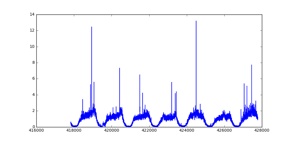
Fig. 1: Normalized session count for a week
Some of those sharp peaks are right after a TV-ad event. Field knowledge says most of the traffic caused by a TV-ad comes up to 8 minutes after the event. I take precaution, and assume some error in reported time of the event. Now let’s remove any reported session from 2 minutes before the event, to 20 minutes after the event. Fig. 2 and 3 show one day of the data, before and after removing data around reported events.
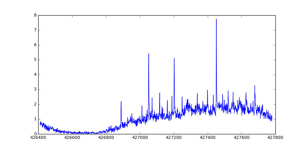
Fig. 2: Normalized session count for a day
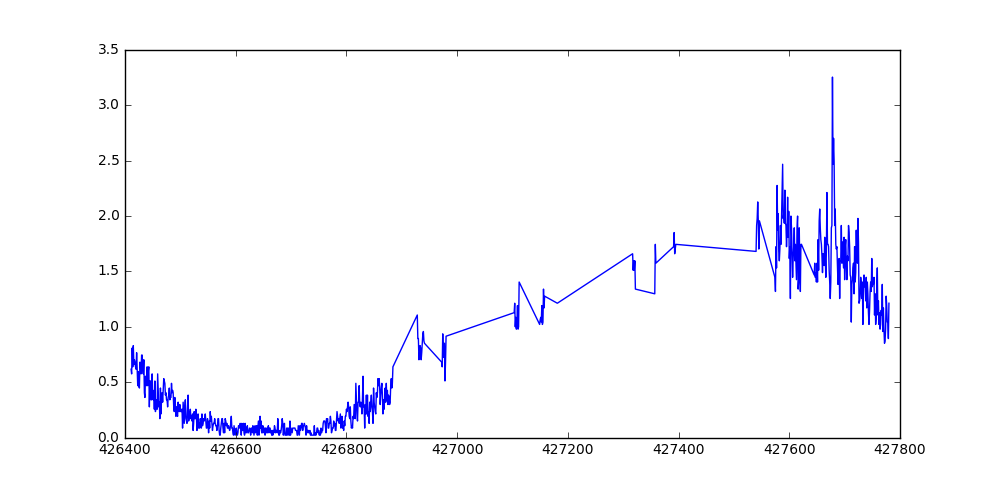
Fig. 3: Normalized session count for a day, after removing data around reported events
Method
Intuitively speaking, I would like to remove the parts of the data close to the given events, fit a model to the remaining data, and then see how close the observed data is to the model’s predictions. If the observed values are significantly higher than the predicted values, most probably some of those sessions are because of the event.
Given an observed and predicted values, deciding whether or not the observed value is significantly larger, can be tricky, and in some cases very arbitrary. Using a method which gives you the probability of an observed value at a given input would make the process much easier. One way of achieving such a goal is to have a method which, intuitively speaking, tells you what it thinks the predicted value is, and also how confident it is. A Gaussian Process (GP) is such a model, in a way that it gives a normal distribution at a given input point as the output. This predicted output has a mean and a variance, which we use to see how probable a given observation is, under the assumption that the model correctly describes the data.
Given a predicted normal distribution, the further the observed value is from the expected mean, the less expected it is. In other words, the larger the blue area shown in Fig. 4, the more probable it’s an outlier.
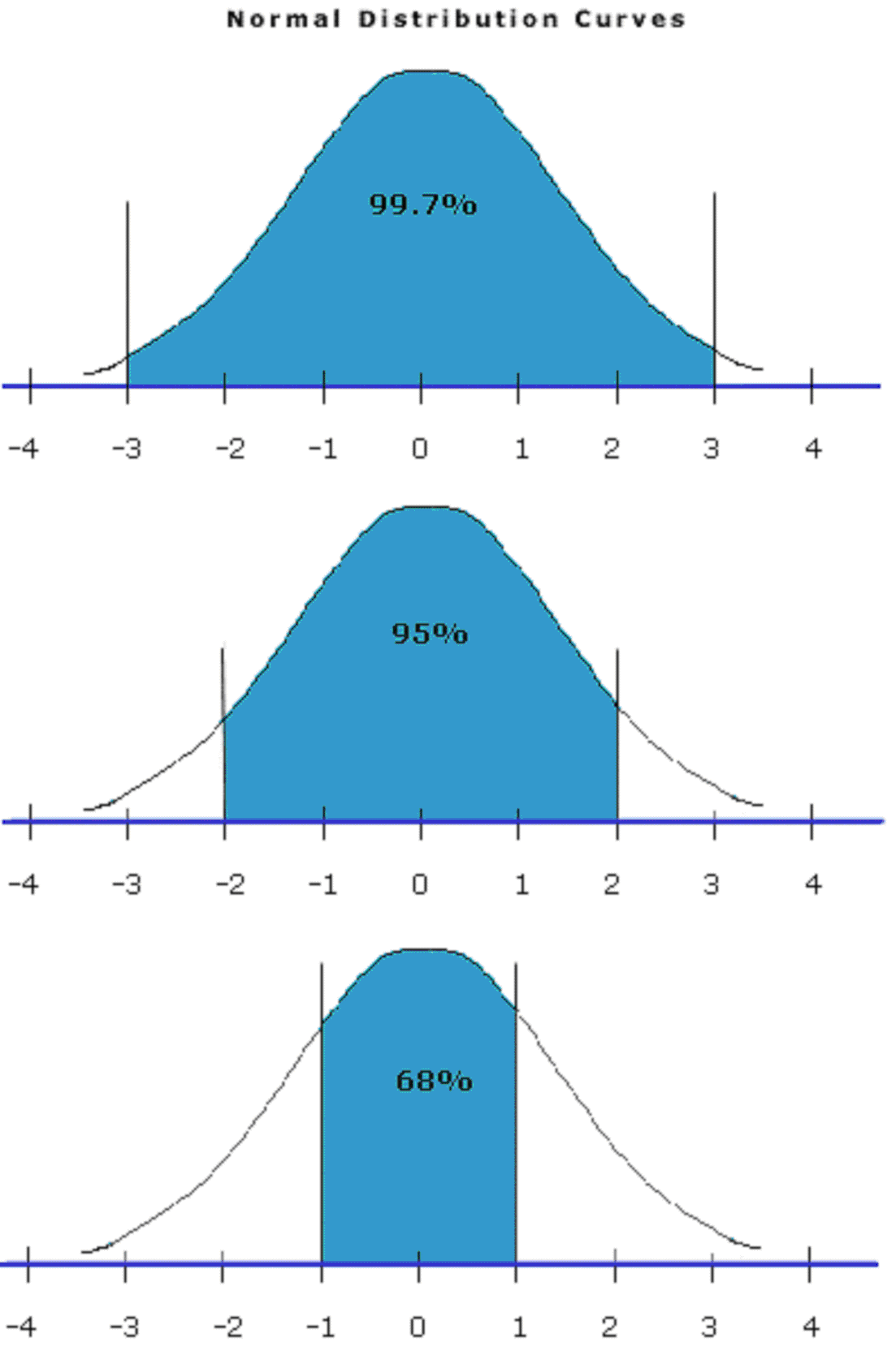
Fig. 4: Normal distribution and three different observed values - credit: thefemalecelebrity.com
The area under the curve marked by the blue areas shown in Fig. 4 is between 0 and 1. It is 0 if the expected value is the same as our observed value, and is close to 1 if it is the two observed and expected mean are far from each other. Hereafter score(x) represents this area under the curve. The piece of code bellow shows how this is calculated in python:
import math
import scipy

def phi(x):
    return 0.5 + 0.5 * scipy.special.erf(x / math.sqrt(2))

def score(x):
    return 1 - abs(phi(x) - phi(-x))

x_score = score((x - expected_mean) / expected_std)
Now for a moment, assume we know a given data point (number of sessions) is influenced by a TV-ad. Still not all those sessions are because of the event. Some of them would have been there even with no TV-ad event. We take the predicted mean as the background session count, and the rest as TV-ad influenced sessions. Therefore, if x is observed value, and x’ is predicted value, (x - x’) / x is the portion of sessions attributed to a TV-ad event.
At the end, we take score(x) * (x - x’) / x as the likelihood of each session being attributed to a TV-ad.
Implementation and Results
I used Python3, matplotlib to generate the plots, and GPy to train the Gaussian Process model.
There are at least two ways of fitting and using GPs in our setting. One is to train a really nice model using the historical data, and use the saved trained model to get predictions for future data. By looking at the data, I would sum these three kernels and optimize on the data:
- A periodic kernel to handle periodicity
- A Gaussian (RBF) kernel to handle the non-periodic part of the data
- A white noise kernel to handle fluctuations seen in the data
Because there were no big enough server available, training a model on the historical data at once was not feasible. Instead, for each day, I take a small part of the data which includes 10 hours before and after start and end of the day, and train a model on that part of the data. This makes training of the model on a small machine feasible, and it also doesn’t require the periodic kernel, which makes the optimization process even faster. Therefore I only use these two kernels:
- A Gaussian (RBF) kernel to handle the non-periodic part of the data
- A white noise kernel to handle fluctuations seen in the data
To summarize, here’s what I do:
- For a given date, take the 44 hours of data corresponding to the given date (10 hours before and 10 hours after the beginning and the end of the day respectively)
- Remove the part of the data around given any TV-ad events in that range.
- Fit a GP to the data.
- Calculate the abovementioned scores for each data point which corresponds to one minute.
Using GPy, I train the model as:
kernel = GPy.kern.RBF(input_dim=1) + GPy.kern.White(input_dim=1)
m = GPy.models.GPRegression(Xtr.reshape(-1,1),ytr.reshape(-1,1),kernel)
m.optimize()
In the above code, Xtr and ytr are the input/output vectors respectively. The Xtr is a sequence of integers representing the minute distance from where the data started, and ytr is the normalized number of sessions for that minute. This results in a model depicted in Fig. 5. The blue gradient represents the variance of the expected output, showing the expected value should be somewhere in the blue region. Please note that we’re only interested in the regions inside the data, and not the region outside the data range.
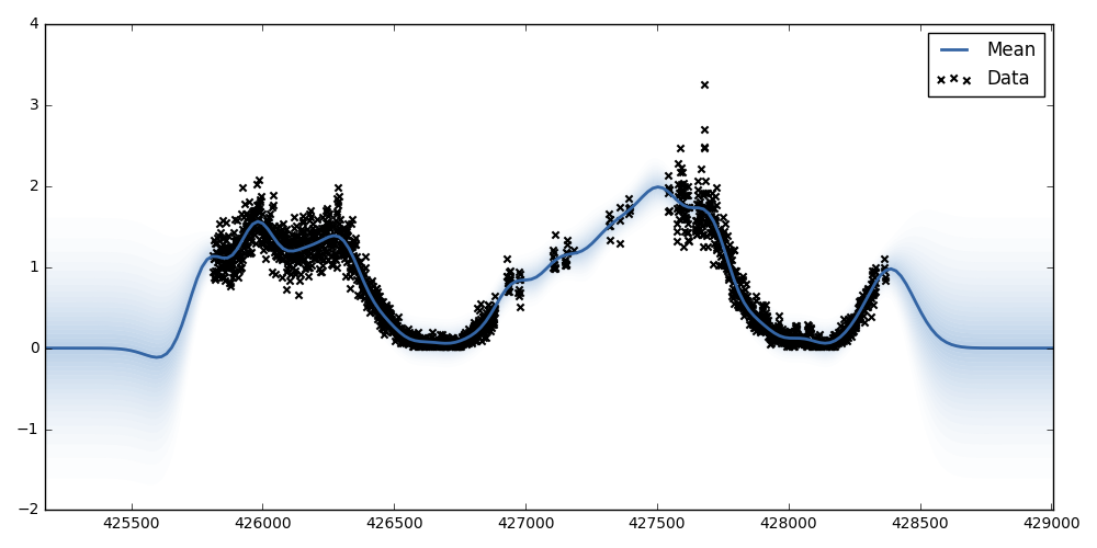
Fig. 5: The trained Gaussian Process model on the 44h of data.
Table 1 shows calculated scores and likelihoods of each session in each minute to be influenced by a TV-ad. A negative portion and likelihood simply mean the expected value is larger that the observed, and can safely be ignored. The Is Significant column simply flags if the score is over 0.9. I would personally attribute only sessions of those minutes to a TV-ad. Also, as expected, not all TV-ad events result in significant rise in the traffic, and some clearly result in more traffic than others.
| Observed | Expected Mean | Expected Variance | Score | Portion | Likelihood | Is Significant | TV-ad |
|---|---|---|---|---|---|---|---|
| 0.96 | 0.84 | 0.03 | 0.52 | 0.12 | 0.06 | ||
| 0.96 | 0.84 | 0.03 | 0.52 | 0.12 | 0.06 | TV | |
| 0.83 | 0.84 | 0.03 | 0.06 | -0.01 | -0.00 | ||
| 0.96 | 0.84 | 0.03 | 0.51 | 0.12 | 0.06 | ||
| 0.81 | 0.84 | 0.03 | 0.16 | -0.04 | -0.01 | ||
| 0.68 | 0.84 | 0.03 | 0.67 | -0.24 | -0.16 | ||
| 0.85 | 0.84 | 0.03 | 0.04 | 0.01 | 0.00 | ||
| 0.72 | 0.84 | 0.03 | 0.52 | -0.17 | -0.09 | ||
| 0.70 | 0.84 | 0.03 | 0.60 | -0.20 | -0.12 | ||
| 1.00 | 0.84 | 0.03 | 0.65 | 0.16 | 0.10 | TV | |
| 1.89 | 0.84 | 0.03 | 1.00 | 0.55 | 0.55 | * | |
| 1.19 | 0.84 | 0.03 | 0.96 | 0.29 | 0.28 | * | |
| 0.94 | 0.85 | 0.03 | 0.41 | 0.10 | 0.04 | ||
| 0.85 | 0.85 | 0.03 | 0.02 | 0.01 | 0.00 | ||
| 0.96 | 0.85 | 0.03 | 0.49 | 0.12 | 0.06 | ||
| 0.83 | 0.85 | 0.03 | 0.08 | -0.02 | -0.00 | ||
| 0.96 | 0.85 | 0.03 | 0.48 | 0.11 | 0.06 | ||
| 1.23 | 0.85 | 0.03 | 0.98 | 0.31 | 0.31 | * | |
| 1.11 | 0.85 | 0.03 | 0.87 | 0.23 | 0.20 | ||
| 0.85 | 0.85 | 0.03 | 0.01 | 0.00 | 0.00 | ||
| 1.04 | 0.85 | 0.03 | 0.74 | 0.18 | 0.14 | TV | |
| 0.77 | 0.85 | 0.03 | 0.38 | -0.11 | -0.04 | ||
| 1.04 | 0.85 | 0.03 | 0.73 | 0.18 | 0.13 | ||
| 1.11 | 0.85 | 0.03 | 0.86 | 0.23 | 0.20 | ||
| 1.13 | 0.85 | 0.03 | 0.89 | 0.24 | 0.21 | ||
| 1.09 | 0.86 | 0.03 | 0.82 | 0.21 | 0.17 | ||
| 1.19 | 0.86 | 0.03 | 0.95 | 0.28 | 0.27 | * | |
| 1.00 | 0.86 | 0.03 | 0.59 | 0.14 | 0.08 | ||
| 0.79 | 0.86 | 0.03 | 0.32 | -0.09 | -0.03 | ||
| 1.11 | 0.86 | 0.03 | 0.84 | 0.22 | 0.19 | ||
| 0.64 | 0.86 | 0.03 | 0.80 | -0.35 | -0.28 | ||
| 0.85 | 0.86 | 0.03 | 0.06 | -0.01 | -0.00 | ||
| 0.96 | 0.87 | 0.03 | 0.41 | 0.10 | 0.04 | ||
| 0.85 | 0.87 | 0.03 | 0.07 | -0.02 | -0.00 | ||
| 0.83 | 0.87 | 0.03 | 0.17 | -0.05 | -0.01 | ||
| 1.34 | 0.87 | 0.03 | 0.99 | 0.35 | 0.35 | * | |
| 0.85 | 0.87 | 0.03 | 0.09 | -0.02 | -0.00 | ||
| 1.17 | 0.87 | 0.03 | 0.91 | 0.25 | 0.23 | * | |
| 0.83 | 0.88 | 0.03 | 0.21 | -0.05 | -0.01 | ||
| 0.77 | 0.88 | 0.03 | 0.48 | -0.14 | -0.07 | ||
| 1.02 | 0.88 | 0.03 | 0.59 | 0.14 | 0.08 | TV | |
| 1.62 | 0.88 | 0.03 | 1.00 | 0.46 | 0.46 | * | TV |
| 1.47 | 0.88 | 0.03 | 1.00 | 0.40 | 0.40 | * | TV |
| 1.26 | 0.89 | 0.03 | 0.97 | 0.29 | 0.29 | * | |
| 1.19 | 0.89 | 0.03 | 0.92 | 0.26 | 0.23 | * | |
| 1.28 | 0.89 | 0.03 | 0.97 | 0.30 | 0.30 | * | |
| 0.91 | 0.89 | 0.03 | 0.11 | 0.03 | 0.00 | ||
| 1.13 | 0.89 | 0.03 | 0.82 | 0.21 | 0.17 | ||
| 1.15 | 0.90 | 0.03 | 0.86 | 0.22 | 0.19 | TV | |
| 4.45 | 0.90 | 0.03 | 1.00 | 0.80 | 0.80 | * | TV |
| 5.40 | 0.90 | 0.03 | 1.00 | 0.83 | 0.83 | * | |
| 3.21 | 0.90 | 0.03 | 1.00 | 0.72 | 0.72 | * | |
| 2.30 | 0.91 | 0.03 | 1.00 | 0.61 | 0.61 | * | |
| 1.96 | 0.91 | 0.03 | 1.00 | 0.54 | 0.54 | * | |
| 1.98 | 0.91 | 0.03 | 1.00 | 0.54 | 0.54 | * | |
| 1.30 | 0.91 | 0.03 | 0.97 | 0.30 | 0.29 | * | |
| 1.47 | 0.92 | 0.03 | 1.00 | 0.38 | 0.37 | * | |
| 0.94 | 0.92 | 0.03 | 0.08 | 0.02 | 0.00 | ||
| 1.00 | 0.92 | 0.03 | 0.35 | 0.08 | 0.03 | ||
| 1.40 | 0.93 | 0.03 | 0.99 | 0.34 | 0.34 | * | |
| 1.30 | 0.93 | 0.03 | 0.97 | 0.28 | 0.28 | * | |
| 1.11 | 0.93 | 0.03 | 0.70 | 0.16 | 0.11 | ||
| 1.00 | 0.93 | 0.03 | 0.30 | 0.07 | 0.02 | ||
| 1.19 | 0.94 | 0.03 | 0.87 | 0.21 | 0.18 | ||
| 1.53 | 0.94 | 0.03 | 1.00 | 0.39 | 0.39 | * | |
| 1.19 | 0.94 | 0.03 | 0.86 | 0.21 | 0.18 | ||
| 1.17 | 0.95 | 0.03 | 0.81 | 0.19 | 0.16 | ||
| 1.17 | 0.95 | 0.03 | 0.81 | 0.19 | 0.15 | ||
| 1.11 | 0.95 | 0.03 | 0.64 | 0.14 | 0.09 | TV | |
| 1.55 | 0.96 | 0.03 | 1.00 | 0.38 | 0.38 | * | TV |
| 2.43 | 0.96 | 0.03 | 1.00 | 0.60 | 0.60 | * | |
| 1.51 | 0.96 | 0.03 | 1.00 | 0.36 | 0.36 | * | |
| 1.62 | 0.97 | 0.03 | 1.00 | 0.40 | 0.40 | * | |
| 1.26 | 0.97 | 0.03 | 0.91 | 0.23 | 0.21 | * | |
| 1.02 | 0.97 | 0.03 | 0.23 | 0.05 | 0.01 | ||
| 1.04 | 0.97 | 0.03 | 0.32 | 0.06 | 0.02 | ||
| 1.19 | 0.98 | 0.03 | 0.80 | 0.18 | 0.14 | ||
| 1.11 | 0.98 | 0.03 | 0.55 | 0.11 | 0.06 | ||
| 0.89 | 0.98 | 0.03 | 0.42 | -0.10 | -0.04 | TV | |
| 1.30 | 0.99 | 0.03 | 0.94 | 0.24 | 0.22 | * | |
| 1.13 | 0.99 | 0.03 | 0.59 | 0.12 | 0.07 | ||
| 1.19 | 0.99 | 0.03 | 0.77 | 0.17 | 0.13 | TV | |
| 1.28 | 1.00 | 0.03 | 0.91 | 0.22 | 0.20 | * | |
| 1.04 | 1.00 | 0.03 | 0.20 | 0.04 | 0.01 | ||
| 1.53 | 1.00 | 0.03 | 1.00 | 0.34 | 0.34 | * | |
| 1.26 | 1.01 | 0.03 | 0.87 | 0.20 | 0.17 | ||
| 1.11 | 1.01 | 0.03 | 0.44 | 0.09 | 0.04 | ||
| 1.34 | 1.01 | 0.03 | 0.96 | 0.24 | 0.23 | * | |
| 1.26 | 1.02 | 0.03 | 0.86 | 0.19 | 0.16 | ||
| 1.04 | 1.02 | 0.03 | 0.11 | 0.02 | 0.00 | ||
| 1.21 | 1.02 | 0.03 | 0.76 | 0.16 | 0.12 | ||
| 1.17 | 1.03 | 0.03 | 0.63 | 0.12 | 0.08 | ||
| 0.81 | 1.03 | 0.03 | 0.83 | -0.27 | -0.23 | ||
| 1.09 | 1.03 | 0.03 | 0.25 | 0.05 | 0.01 | ||
| 1.23 | 1.04 | 0.03 | 0.78 | 0.16 | 0.13 | ||
| 1.36 | 1.04 | 0.03 | 0.96 | 0.24 | 0.23 | * | |
| 0.87 | 1.04 | 0.03 | 0.71 | -0.20 | -0.14 | ||
| 1.09 | 1.05 | 0.03 | 0.19 | 0.04 | 0.01 | ||
| 1.00 | 1.05 | 0.03 | 0.24 | -0.05 | -0.01 | ||
| 1.36 | 1.05 | 0.03 | 0.95 | 0.23 | 0.22 | * | |
| 1.30 | 1.05 | 0.03 | 0.87 | 0.19 | 0.16 | ||
| 1.15 | 1.09 | 0.02 | 0.32 | 0.06 | 0.02 | ||
| 1.26 | 1.09 | 0.02 | 0.72 | 0.13 | 0.10 | ||
| 1.40 | 1.09 | 0.02 | 0.96 | 0.22 | 0.21 | * | TV |
| 2.57 | 1.09 | 0.02 | 1.00 | 0.58 | 0.58 | * | |
| 2.77 | 1.10 | 0.02 | 1.00 | 0.60 | 0.60 | * | TV |
| 1.51 | 1.10 | 0.02 | 0.99 | 0.27 | 0.27 | * | |
| 1.30 | 1.10 | 0.02 | 0.80 | 0.15 | 0.12 | ||
| 1.34 | 1.10 | 0.02 | 0.87 | 0.18 | 0.16 | ||
| 1.30 | 1.10 | 0.02 | 0.79 | 0.15 | 0.12 | ||
| 1.06 | 1.11 | 0.02 | 0.21 | -0.04 | -0.01 | ||
| 1.30 | 1.11 | 0.02 | 0.78 | 0.15 | 0.11 | ||
| 1.19 | 1.11 | 0.02 | 0.40 | 0.07 | 0.03 | ||
| 1.23 | 1.11 | 0.02 | 0.56 | 0.10 | 0.06 | ||
| 1.19 | 1.11 | 0.02 | 0.38 | 0.06 | 0.02 | ||
| 1.40 | 1.12 | 0.02 | 0.94 | 0.20 | 0.19 | * | |
| 1.00 | 1.12 | 0.02 | 0.55 | -0.12 | -0.07 | TV | |
| 1.32 | 1.12 | 0.02 | 0.80 | 0.15 | 0.12 | TV | |
| 1.87 | 1.12 | 0.02 | 1.00 | 0.40 | 0.40 | * | |
| 1.62 | 1.12 | 0.02 | 1.00 | 0.31 | 0.30 | * | |
| 1.36 | 1.13 | 0.02 | 0.87 | 0.17 | 0.15 | ||
| 1.06 | 1.13 | 0.02 | 0.32 | -0.06 | -0.02 | ||
| 0.96 | 1.13 | 0.02 | 0.73 | -0.18 | -0.13 | ||
| 1.72 | 1.13 | 0.02 | 1.00 | 0.34 | 0.34 | * | |
| 1.06 | 1.13 | 0.02 | 0.34 | -0.06 | -0.02 | ||
| 1.28 | 1.13 | 0.02 | 0.64 | 0.11 | 0.07 | ||
| 1.04 | 1.13 | 0.02 | 0.45 | -0.09 | -0.04 | ||
| 1.28 | 1.14 | 0.02 | 0.63 | 0.11 | 0.07 | ||
| 1.34 | 1.14 | 0.02 | 0.81 | 0.15 | 0.12 | ||
| 1.26 | 1.14 | 0.02 | 0.55 | 0.09 | 0.05 | ||
| 1.21 | 1.14 | 0.02 | 0.36 | 0.06 | 0.02 | ||
| 1.26 | 1.14 | 0.02 | 0.54 | 0.09 | 0.05 | ||
| 1.40 | 1.14 | 0.02 | 0.91 | 0.19 | 0.17 | * | |
| 1.00 | 1.14 | 0.02 | 0.64 | -0.14 | -0.09 | ||
| 0.98 | 1.14 | 0.02 | 0.71 | -0.17 | -0.12 |
Table 1: A piece of output of the method